This post explains all the key concepts of optimization in Machine learning and deep dives into SGD along with mathematical derivation and code implementation of the same in Keras python module.

Introduction to gradient descent

Okay so generally in machine learning you have some training dataset on which you are supposed to build a model so as to predict or classify some properties learned from the dataset.

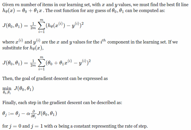
For which we have some terms called parameters which are basically forms you the mathematical model or hypothesis equation. There can be multiple hypothesis equations for different parameters producing different output. But we are interested in one such hypothesis equation which will best fit our dataset in the perfect manner in order to make real-time decision.

Now comes the question of how can we find our optimum model for that we have cost functions.

A cost function basically is way to determine how accurate your model is or if I put it better way it tells you difference between your models output and the desired output. We basically want our cost function to be zero, in other ways we can say that we want to minimize our cost function.

As the parameters increases the model becomes more complex and the combinations of parameters also increases exponentially. In this case it would be really difficult to try out all the model outputs and determine the local minimum.

So people felt there’s a need for a software or an algorithm which can automatically take us to the local minimum, that’s when Gradient descent came into picture.

Gradient descent basically decreases or increases the values of the parameters of your model in order to reach the local minimum faster without trying out values of all the parameters (which would be a huge combination), so the gradient descent uses a learning rate (alpha) which basically is a multiplier which lets you reach the local min faster.

Selection of a smaller value will lead to local minimum slower or a higher value will lead to oscillation of the final cost functions.

Main Formulas

Below are the list of formulas which is developed in the DeepRust project.

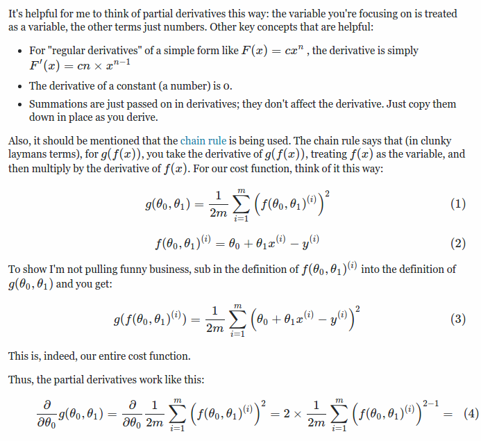
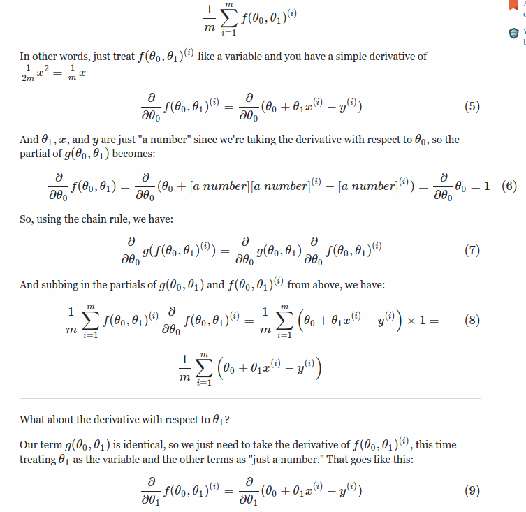
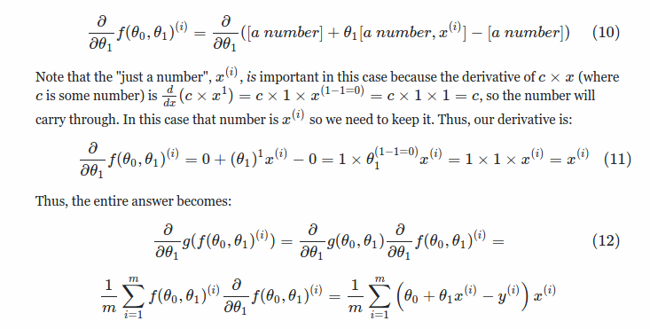
Mathematical derivations

The below derivations are how we arive at the mathematical formulas above.

Stochastic gradient descent

Stochastic gradient descent is commonly reffered to as SGD, going ahead I will be using the short form only. The above method of gradient descent is called as Batch gradient descent, where the whole training data is given as the input to the network and back propagated well this works good for smaller dataset but while we scale up the model we face the following problems:

• Computation Inability Its likely that you would be designing a model to solve a real world problem where there’s amaple amount of data ans conditions and its not possible to load the complete data in the RAM of the hardware. The computation cost associated with running training on the complete data sets is not possible in real life scenarios as the datasets are huge.

• Slow Since we are running the training on the complete dataset in gradient descent, it is very slow as the backpropogation takes time.

What SGD offers is that, it takes mini batches of data for training and updates the weight after back propogation of the first minibatch and so on. This ideas solves us a lot of problems about harware resources as mentioned below,

• This process allows the hardware to exploit the highly optimized matrix operations of cost and gradient, so we will have computation problems
• This reduces the variance in the parameter update and can lead to more stable convergence, as the learning rate is very less than the

Note: A typical minibatch size is 256, although the optimal size of the minibatch can vary for different applications and architectures.

In SGD the learning rate α is typically much smaller than a corresponding learning rate in batch gradient descent because there is much more variance in the update.

θ=θ−α∇θJ(θ;x(i),y(i))

Choosing the proper learning rate and schedule (i.e. changing the value of the learning rate as learning progresses) is a fairly difficult task. One standard method that works well in practice is to use a small enough constant learning rate that gives stable convergence in the initial epoch (full pass through the training set) or two of training and then halve the value of the learning rate as convergence slows down.

An even better approach is to evaluate a held out set after each epoch and anneal the learning rate when the change in objective between epochs is below a small threshold. This tends to give good convergence to a local optima. Another commonly used schedule is to anneal the learning rate at each iteration t as a/(b+t)

where a and b dictate the initial learning rate and when the annealing begins respectively.

If the data is given in some meaningful order, this can bias the gradient and lead to poor convergence. Generally a good method to avoid this is to randomly shuffle the data prior to each epoch of training.

Momentum

The objective of the optimization function has always been to reach the optimal minima but in most of the cases of standard SGD they tend to oscillate across the narrow minima values as the negative gradient will point down one of the steep side rather than along the ravine towards the optimum.

The objectives of deep architectures have this form near local optima and thus standard SGD can lead to very slow convergence particularly after the initial steep gains. Momentum is one method for pushing the objective more quickly along the shallow ravine. The momentum update is given by,

v = γv+α∇θJ(θ;x(i),y(i))
θ = θ−v

In the above equation v is the current velocity vector which is of the same dimension as the parameter vector θ. The learning rate α is as described above, although when using momentum α may need to be smaller since the magnitude of the gradient will be larger. Finally γ∈(0,1] determines for how many iterations the previous gradients are incorporated into the current update. Generally γ is set to 0.5 until the initial learning stabilizes and then is increased to 0.9 or higher.

Code implementation

Keras Implementation

• Create a file name sample_sgd.py

• Copy paste the code below

#importing the keras Deeplearning library
from keras import optimizers

#Creating a new object 
model = Sequential()

#Dense - Regular densely-connected NN layer
model.add(Dense(64, init='uniform', input_shape=(10,)))

#Applying the other stacked layers
model.add(Activation('tanh'))
model.add(Activation('softmax'))

#Defined the SGD optimizer with a learning rate of 1e-16 and momentun of o.9
sgd = optimizers.SGD(lr=0.01, decay=1e-6, momentum=0.9, nesterov=True)
model.compile(loss='mean_squared_error', optimizer=sgd)

#x_train and y_train are Numpy arrays -- traning dataset
model.fit(x_train, y_train, epochs=5, batch_size=32)

#or 
#model.train_on_batch(x_batch, y_batch)

#Evaluating metrics
loss_and_metrics = model.evaluate(x_test, y_test, batch_size=128)

#Predic the class at realtime
classes = model.predict(x_test, batch_size=128)

• For running,

python sample_sgd.py

Ref:

• Difference between SGD and GD
• Derivation
• Code - Keras
• Code - Tensorflow
• SGD